In [1]:
from __future__ import division
from iirrational.utilities.ipynb_lazy import *
Populating the interactive namespace from numpy and matplotlib
Random Filter fit with comparison
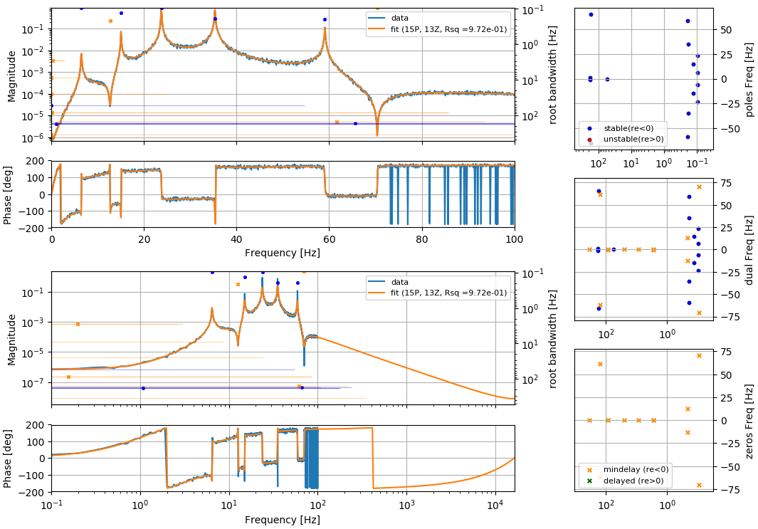
Show stage-1 Rational Disc Fit
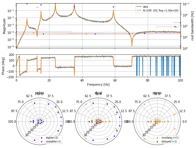
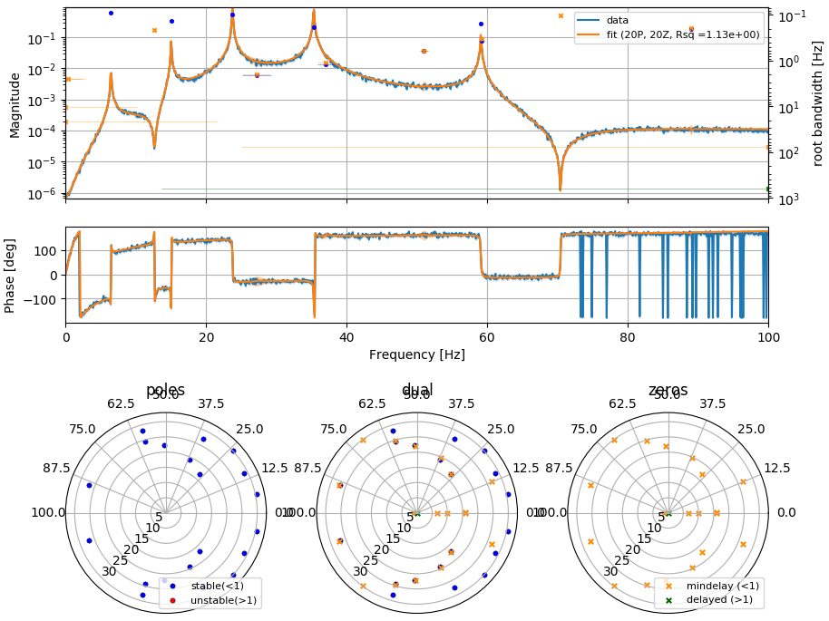
Here is the preliminary fit on a reduced-nyquist disc
The poles and zeros are shown on the full disc. Note that unstable poles are allowed on the real line as these are removed by analytic surgery during the nyquist shift
In [6]:
dat = iirrational_data('rand10_lin1k', set_num = 5)
out = v1.rational_disc_fit(
    dat,
)
ax = plot_fitter_flag(out)
(direct = 4.164e+00, Psvd= 4.164e+00, Zsvd= 4.164e+00)
LINEAR Final Residuals:  3.95445037567
(direct = 3.930e+00, Psvd= 3.930e+00, Zsvd= 3.930e+00)
LINEAR Final Residuals:  3.93098246203
Using last (reduced)! 20
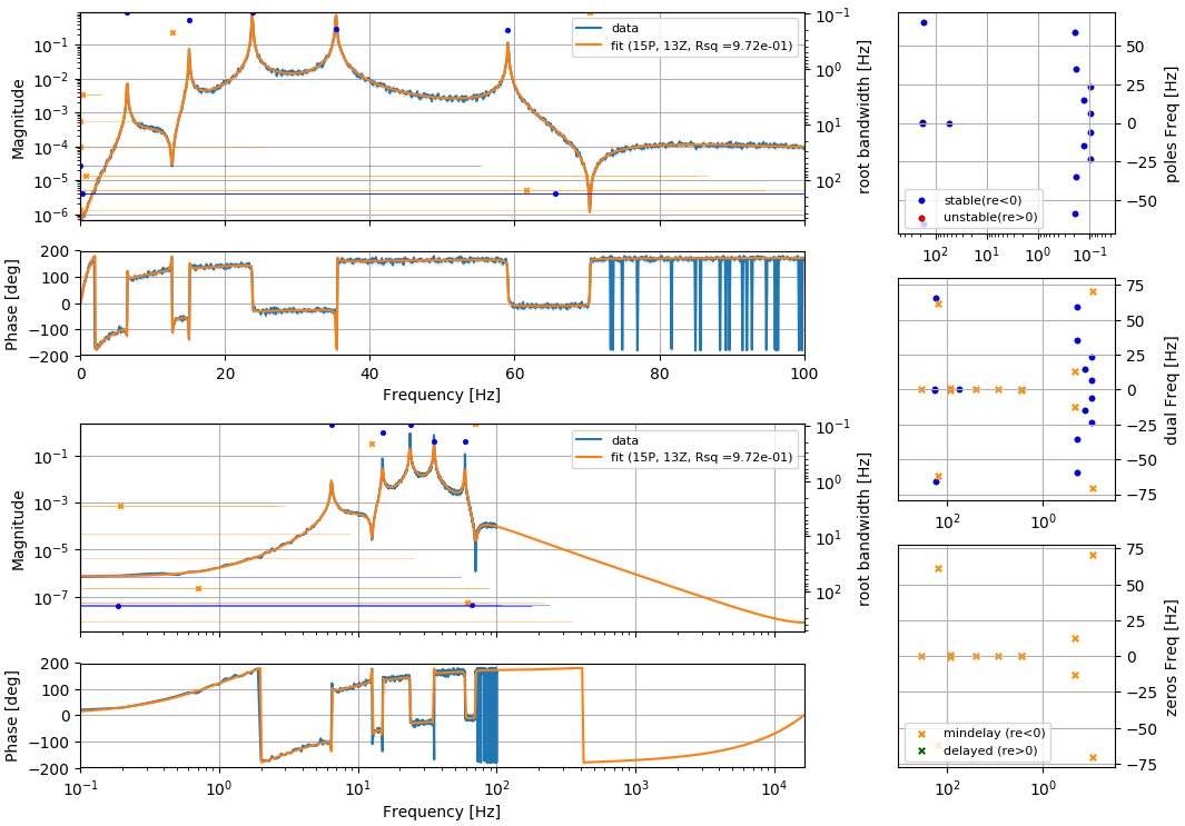
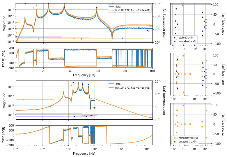
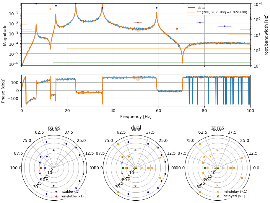
With nyquist shift
The data detunes from being a great fit
In [7]:
dat = iirrational_data('rand10_lin1k', set_num = 5)
out = v1.rational_disc_fit(
    dat,
    nyquist_final_Hz = 16384,
)
ax = plot_fitter_flag(out)
(direct = 4.164e+00, Psvd= 4.164e+00, Zsvd= 4.164e+00)
LINEAR Final Residuals:  3.95445037567
(direct = 3.930e+00, Psvd= 3.930e+00, Zsvd= 3.930e+00)
LINEAR Final Residuals:  3.93098246203
Using last (reduced)! 20
Cleared  pole (-1.04899302868+0j)
Cleared  zero (-7.22335881797+0j)
Cleared  zero (-1.05198172682+0j)
Cleared  zero (-0.584295509961+0j)
In [8]:
%%time

out = v1.data2filter(
    dat,
    delay_s = None,
)
(direct = 4.164e+00, Psvd= 4.164e+00, Zsvd= 4.164e+00)
LINEAR Final Residuals:  3.95445037567
(direct = 3.930e+00, Psvd= 3.930e+00, Zsvd= 3.930e+00)
LINEAR Final Residuals:  3.93098246203
Using last (reduced)! 20
Cleared  pole (-1.04899302868+0j)
Cleared  zero (-7.22335881797+0j)
Cleared  zero (-1.05198172682+0j)
Cleared  zero (-0.584295509961+0j)
Initial Order: (Z= 17, P= 19, Z-P= -2)
TRIPLETS (rat = 1.0010150038962191, pre = 0.9734729303474599, mid = 0.9734729249578383, post = 0.9734722105759255
N:  2
RATIO:  10.9002733839
fit NOT improved from pair at 13.8397945578
RATIO:  18.3818734556
fit NOT improved from pair at 9.56094083217
RATIO:  10.7017576506
fit NOT improved from pair at 18.2046398213
RATIO:  1.03476207996
fit NOT improved from pair at 64.7360498735
[0.96102176342334822] zeros
[(0.98751653189313626+0.0050603760550500913j), (0.98751653189313626-0.0050603760550500913j)] zeros
[0.98726211674090025] poles
[(0.97815059543903571+3.9610796052692903e-05j), (0.97815059543903571-3.9610796052692903e-05j)] poles
WEAK REMOVE:  [(0.98751653189313626+0.0050603760550500913j), (0.98751653189313626-0.0050603760550500913j)] [(0.97815059543903571+3.9610796052692903e-05j), (0.97815059543903571-3.9610796052692903e-05j)]
RATIO for WEAK:  1.00330207037
FINAL RESIDUALS 0.970649728969
CPU times: user 16.3 s, sys: 34 s, total: 50.2 s
Wall time: 15.8 s
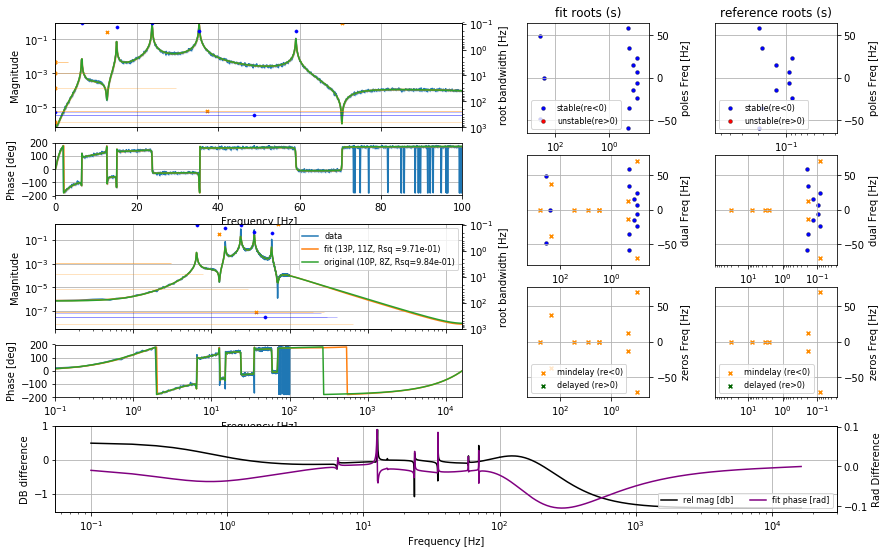
In [10]:
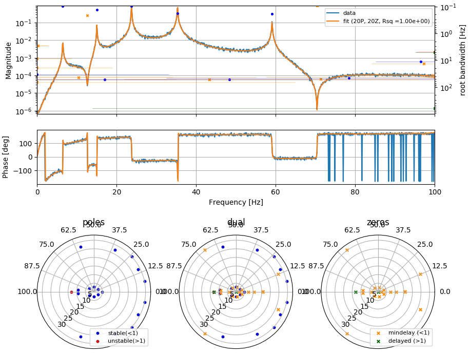
ax = plot_fitter_flag_compare(out.fitter, dat.fitter)
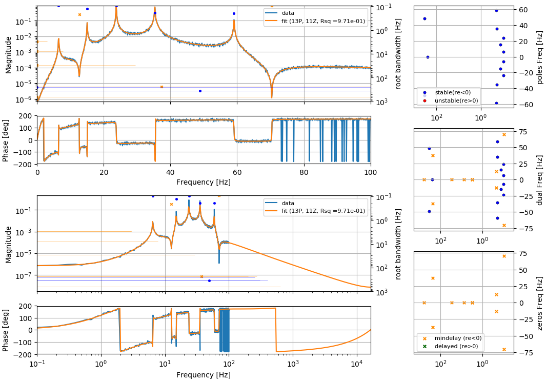
In [12]:
out.digest_write(
    folder = 'random',
    clear_plots = True,
    ipy_display = True,
    MP_workers = 1,
)
REMOVING:  random/plot-main
REMOVING:  random/plot-1
PLOTTING:  random/plot-1-1
PLOTTING:  random/plot-1-2
PLOTTING:  random/plot-1-3
REMOVING:  random/plot-1-4
PLOTTING:  random/plot-1-5
PLOTTING:  random/plot-1-6
PLOTTING:  random/plot-1-7
PLOTTING:  random/plot-2
PLOTTING:  random/plot-3
REMOVING:  random/plot-4
PLOTTING:  random/plot-4-1
PLOTTING:  random/plot-4-2
REMOVING:  random/plot-5
REMOVING:  random/plot-6
REMOVING:  random/plot-7
REMOVING:  random/plot-8
REMOVING:  random/plot-9
PLOTTING:  random/plot-10
fit_sequence version 1
v1.fit_sequence
Version 1 smart fitter in iirrational library. Uses SVD method with high order over-fitting, then switches to nonlinear fits with heuristics to remove poles and zeros down to a reasonable system order.
1 initial
1.4 choose zeros
if
Chose the zeros SVD fitter as it had the smaller residual of 4.04e+00 vs. 4.46e+00 for the poles
1.5 seq_iter_3
RationalDiscFilter.fit_poles, RationalDiscFilter.fit_zeros
First iterations, enforcing stabilized poles residual of 3.95e+00
1.6 seq_iter_4
RationalDiscFilter.fit_poles, RationalDiscFilter.fit_zeros
First iterations, enforcing stabilized poles residual of 3.95e+00

1.7 Final
SVD_method
create initial guess of fit for data, followed by several iterative fits (see reference ???). * It is a linear method, finding global optimum (nonlocal). This makes it get stuck if systematics are bad. To prevent this, it requires gratuitous overfitting to reliably get good fits. * It requires a nyquist frequency that is very low, near the last data point. This can cause artifacts due to phasing discontinuity near the nyquist. * The provided nyquist frequency is shifted up at the end, removing the real poles/zeros that are typically due to phasing discontinuity
2 nonlinear pre-reduce and optimize
MultiReprFilter.optimize
initial conservative order reduction (for speed), followed by a nonlinear optimization.
3 optimize nonlinear after bandwidth limiting
MultiReprFilter.optimize
ths limited in the nonlinear representation to half of the local average the frequency spacing. Nonlinear optimization then applied.