Quickstart¶

Install IIRrational through pip as a first step. Be sure to run pip from the environment you will be using IIRrational from.

First Fit¶

As seen in the introduction page, the minimal code to fit and see it is:

import iirrational.v1
import iirrational.plots
from iirrational.testing import iirrational_data

dataset = iirrational_data('simple2')
fit = iirrational.v1.data2filter(
    data = dataset.data,
    F_Hz = dataset.F_Hz,
    SNR  = dataset.SNR,
    F_nyquist_Hz = 16384,
)

#see the ZPK generated (Z-domain with the provided Nyquist frequency)
print(fit.fitter.ZPK)

#plot the output
ax = iirrational.plots.plot_fitter_flag(fit.fitter)

This example shows a few notable aspects of the library.

The main fitter code is in a “v1” submodule. This is to provide some versioning between the methods and heuristics used. Hopefully the library becomes monotonically better, but without a formal problem statement, that is impossible to define.

For this reason, the composite all-in-one fitting methods will be versioned. For versions greater than the current library version, the API and heuristics will not be stable, for version submodules equal or below the library version, it should remain stable (this may require migrating common code into the submodule as common code changes).

The return object is composite, with a “fitter” attribute holding the current best fit, the data, SNR and everything in the plot.
A Nyquist frequency is required. This should be one half the sample frequency. Currently S-domain output is not supported (will be in the future). The ZPK output
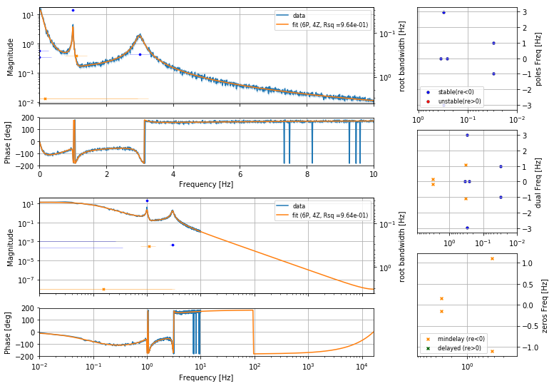
Plotting functions are provided to conviently assess the quality of fit. The “flag” plots show top-left a zoom to the data, linear if the data is linear spaced, and log otherwise.

The lower left is a zoom out to the Nyquist frequency to see if the rolloff is well-matched. Since this is Z-domain the phase will always reture to 0 or 180 at the Nyquist (thanks Cauchy). The right line are Pole, PZ, Zero plots in the S-domain (really the Z-domain zoomed in near 1 and conformally remapped..). These are also overlayed in the loglog plots using the right y-axis. These plots are log-scaled in the bandwidth (S root real) and right-plane roots are mirrored and recolored.
The library includes some example data generators through the testing submodule

Example Data¶

Example data generators are useful for the test-suite and for this documentation. Most of them are randomly generated filters multiplied by noise consistent with a constant SNR. These data are very well behaved compared to real data in having constant, well-estimated SNR. If the library is run from its development folder, an additional module iirrational_test_data is available with contributed real data test cases. To reduce size these are not distributed through pip/setuptools.

You can see the available cases at

internal https://github.com/mccullerlp/iirrational/blob/master/iirrational/testing/__init__.py

contrbuted https://github.com/mccullerlp/iirrational/blob/master/iirrational_test_data/__init__.py

these are accessed through the functions iirrational.testing.iirrational_data() and iirrational_test_data.iirrational_data_dev() using a keyword set name. The random sets also take a set_num argument and instance_num. For the random sets, the set_num changes the last data point (10Hz to 100Hz) and also linear vs. log distribution. The instance number seeds the random noise added, so that the fitting is deterministic for a given instance.

The data2filter() function can take as its first positional argument a dictionary with the other keywords. This allows the sets to be fit and tested using only:

import iirrational.v1
import iirrational.plots
from iirrational.testing import iirrational_data

fit = iirrational.v1.data2filter(
  iirrational_data('simple2'),
)
ax = iirrational.plots.plot_fitter_flag(fit.fitter)

Fitting¶

iirrational.v1.data2filter()¶

Fits frequency-response data using 2-stage process

Parameters:

argB (Mapping) – optional positional argument with dict-like full of keyword arguments. Explicit arguments supercede the ones provided by this argument.
data (ndarray) – Complex array containing transfer-function to fit.
F_Hz (ndarray) – Real array with frequency points of each data point.
SNR (ndarray or float) – Array of weights for the data. May be a single value. Zeros allowed, NaN’s and infinities will break the fit.
F_nyquist_Hz (float) – Value to use for Nyquist frequency of Z-domain representation.
ZPK ([Z-tuple, P-tuple, float]) – Optional! If provided, the stage-1 will be skipped and only the nonlinear fitting and order reduction will be applied
order_initial (int) – Optional order to stage-1 fitting. If not provided the order is scaled up exponentially until residuals stabilize. This should be higher than the known system order as stage-1 warps the domain and needs extra order to compensate for systematics.
SNR_cutoff (float) – defaults to 100. Clips SNR to prevent over-emphases on featureless parts of the data. Coherence SNR estimates can over-weight data.
delay_s – If None the delay is fit out near the end. This is often degenerate with the fit order unless the data extends to high frequencies. Use 0 otherwise. Not yet implemented is to use the specified value
hints (dict or list-of-dicts) – Hierarchical hint keywords to affect internal algorithms, verbosity, and more.

Returns:

FitAid collection

Fitter Output (FitAid)¶

The output of the fitter is a container that holds the best fit, the hint dictionary, some methods used for evaluating fits, and the annotation log. All of the internal algorithm functions interface with it for settings and to store their improvements to the fit. As a user, only the stored fits are useful. In the future some interfaces for finding hints and their default values and hierarchy will be exposed.

The additional fitters stored which have the lowest residuals seen are usable during the order-reduction algorithm for robust statistics as to how well the fitting CAN do vs. what is sacrificed by order reduction.

class v1.FitAid¶

Stores and exposes the output of fitting algorithms. Exposed attributes to use are:

fitter¶: A MultiReprFilter (MRF) Object with the current best fit. This object exposes the current residuals, errorbars and parameterization. The most immediately useful attribute of it is ZPK to get the Z-domain root.

fitter_lowres_avg¶: MRF type with the lowest average residuals seen (may not be order-reduced).

fitter_lowres_max¶: MRF type with the lowest max (L-infinity) residuals seen (may not be order-reduced).

fitter_lowres_med¶: MRF type with the lowest median residuals seen (may not be order-reduced).

fitter_loword¶: MRF type with the lowest order seen.

digest_write()¶: method to write a digest of the algorithm internals (described below).

Hints¶

The algorithms internally use a hierarchical hinting system to adjust thresholds and settings. The semantics for these hints are not yet well established, but some useful ones are:

log_print: Specify whether to print log output. Set to False to reduce the stuff printed (which is internal algorithm diagnostics)
optimize_log: Whether to log on the MultiReprFilter.optimize() calls. Gives the nonlinear optimizer termination conditions, be they ftol, xtol, gtol, ran past maxfevs and such.
optimize_max_nfev: The number of function evaluations allowed during a nonlinear optimization call
optimize_ftol: The relative tolerance in the nonlinear optimization calls. Set larger to trade speed for accuracy (the default has not be tuned)
resavg_RthreshOrdDn: The relative threshold on the ratio of the new residual chi-sqaure from a previous residual for an order reduction. Defaults to 1.10. Increase for more aggressive reduction
resavg_RthreshOrdUp: relative threshold for heuristics that increase the order. Defaults to 1 but less may make sense
resavg_RthreshOrdC: relative threshold for heuristics that preserve the order.
resavg_EthreshOrdDn: threshold for the Exact residual average value to accept an order reduction. Makes sense for data without noise where the residual is numeric precision or exactness-of-representation limited (designed in S, fit in Z for example)

The can be specified in a dictionary, and there is a collection of “good” sets for specific purposes. An example usage for a quiet exact fit is.

import iirrational.v1
import iirrational.plots
from iirrational.testing import iirrational_data

fit = iirrational.v1.data2filter(
  iirrational_data('simple0E'),
  SNR = 1,
  hints = [
      {'resavg_EthreshOrdDn': 0.1,
       'resavg_RthreshOrdC':  None,
       'resavg_RthreshOrdDn': None,
       'resavg_RthreshOrdUp': None},
      iirrational.v1.hintsets.quiet,
  ]
)
ax = iirrational.plots.plot_fitter_flag(fit.fitter)

Gotchas¶

Since this library attempts to forgo initial guesses, it must have some basis for order estimation. This means that for datasets with features that haven’t been tested against, the fitter may give objectionable fits, often missing features because its initial order was too low or its reduction heuristics too aggressive.

Generally the fits are improved if order_initial is specified with a large value. 50-100 roots is a benchmark that seems to always get good fits, much larger and the fits slow down and become numerically less stable. The downside is that this slows down fits that don’t need it, and the order reduction has to work harder, and it is not yet particularly effective.

Plotting¶

Todo

More docs of the various plotters, how to save and how to enable/disable automatic interactive plots (particularly for matlab users).

Annotated Digest¶

The data2filter output FitAid object can output a digest with plots of the internal steps of the algorithm. This is mostly useful for developing the heuristics, but useful to tech some methods. Could be used to generate logbook posts. Inspect the code behind data2filter to learn how to use it.

See the end of the Random Filter fit with comparison note for an example call. And the digest output can be seen in the notebook as it uses the ipy_digest argument.

iirrational.v1.FitAid.digest_write()¶

Write a digest of the fit algorithm in Markdown

Parameters:

folder – First positional with the folder to dump the plots and markdown file
format – Currently must be the (default) “Markdown”
md_name – Name of the markdown file within the folder. Defaults to “digest.md”
plot_verbosity – Verbosity tags above this will not be plotted
md_verbosity – Verbosity tags above this will not have a section
clear_plots – Delete original plots if not over-plotted
regex_plotsections – Only plot in sections meeting this regex (for algorithm debugging)
ipy_display – Dump the markdown into the ipython notebook
plot_format – Format to write the plots. Default is “png”. Pdf is possible but most markdown renderers don’t support it.
dpi – DPI for plots
MP_workers – 1 is default. If larger it uses multiprocessing. Matplotlib sometimes misbehaves and clips plots strangely when above 1.

Contributing Testcases¶

To improve the library, more examples of real-world usage are needed. A function call with nearly the same interface as data2filter() exists for this purpose. Please email, add an issue or pull request with collections of data. The Matlab format from this is relatively compact and easy to read, so please use this function to provide data. If you have larger test-suites for evential MIMO or Feedforward testing, hdf5 format is preferred but a standard layout has not yet been established.

iirrational.v1.data2testcase()¶

Store fit-data in a common format for inclusion into the test-suite

Parameters:

argB – mapping of arguments for packaged data
data – complex array to fit
F_Hz – array of frequencies for data
SNR – float or array of SNR weights
fname – filename to write. Should include the “.mat” format
F_nyquist_Hz – Optional but highly recommended best nyquist frequency for problem domain. Used when a Z bestfit ZPK is provided.
bestfit_ZPK_z – Optional ZPK in Z domain with a reference fit to compare against. Should be a “good” fit, rather than a failed output of data2filter.
bestfit_ZPK_s – Optional ZPK in S domain with a reference fit to compare against. Should be a “good” fit.
F_ref_Hz – Reference frequency for S-to-Z conversion. Defaults to 0 but this is inappropriate for high-DC-gain filters.
description – A description of the dataset source, aspects to preserve or anything of relevance for testers.

Example Notebooks¶

Use the “view page source” link at the top to download the original .ipynb file to run yourself.